3 things that are not so impressive in Excel 2013

The whole cloud thing:

While it is understandable that Microsoft wants us all to purchase shiny new Surface tablets and use spreadsheets on the go, it seems like a bad idea. It annoys me that when I want to save a file, the first option I see is Kokula Krishna Hari K’s sky drive. The process of saving files to sky drive and later viewing them in browsers is very slow and often results in errors or warnings. Instead, for desktop versions, why not make My computer as first preference?!?

Sharing & Social features:

Share to Facebook?!? seriously! Why would anyone want to share their spreadsheets on twitter or facebook? Do we really want facebook to know our annual budget & appraisal ratings (so that they can show us ads that say –Buy our scissors and cut your budget in half )?

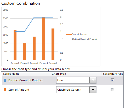
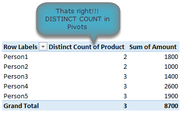
Power Pivot is not for masses:

Microsoft positioned Power Pivot as BI for masses, offered it for free in Excel 2010. Then in Excel 2013, they went ahead and implemented a licensing policy that looks just as complicated as my lawyer’s invoice. Why would a for-profit company like MS want to not offer powerful tools like Power Pivot to masses for a fee? Why sell it only to corporate customers through volume licensing program? beats me.

Bottom line

Despite these minor annoyances, I think Excel 2013 is a well designed, solid & powerful software ready to make more people awesome in their work. With features like tablet compatibility, data model, slicers & timelines, improved UI & color schemes it has quickly become my first choice when I want to use a spreadsheet (I run Excel 2010 & 2013 on same computer).

Easier Charting

In Excel 2013, there are massive changes in charting. Now you can create combination charts, add secondary axis, set up smart data labels, format the chart or switch styles with ease. Microsoft revamped the default formats too so that when you make a chart from data, it is ready for presentation (with out too many tweaks).

Some of favorite charting features are,

• Recommended charts feature that tells you which charts go well with your data.
• A screen where you can change the chart type for each series easily.
• Common chart customizations are a click away
• Ability to create scatter plots based on a variety of input data layouts.

That said not everything is rosy with 2013 charting. For example, I do not like that we have to go through sidebar pane to customize charts (formatting etc.) instead of dialog box.

Distinct Counts & more in your Pivot

If you are really quiet, you can hear an analyst in your company screaming with joy once they realize that in Excel 2013, you can get distinct count of values in pivot reports!!!

That is right, using Excel 2013 pivot reports, you can find out distinct counts. No extra formulas or no arrays or no VBA.

Timelines - New Feature in Excel 2013

These days everybody boasts of a massive spreadsheet. But almost no one needs all the data at same time. We are always filtering data for latest quarter, 6 months starting Mother’s day or 8 weeks from November 1st etc. Of course, you can use auto-filter and select all the dates. But it is a pain.

Thanks to Timelines,  filtering for dates is a breeze. You can add timelines for any date column in a pivot table / pivot chart. I am sure your clients & bosses will love it.

Flash Fill - Microsoft Office Excel 2013

Imagine Flash (the super hero, not browser add-in) is using Excel to extract the middle names of all his villains. Now, flash being flash, do you think he will slowly type out the middle names one at a time? Of course, he can learn Excel formulas and do it in one stroke. But he is too busy running around & saving earth. So, obviously he would use Flash Fill.

Flash Fill works almost like magic. It looks at what you are typing and sees if there is any pattern in it (based on adjacent columns etc.) and then suggests a fill down option. See this demo.

Shortcut Key : Press CTRL+E to activate flash fill.

Autonumbering in Excel 2013

It is often useful to number the rows in an Excel spreadsheet as a means to help organize your data, much in the same way that column heading are added.

There is very quick and simple way to number rows, and it doesn’t involve any math formulas or special tricks. Let’s begin with the example shown in Picture One.

Figure 1 - Excel with Filled Series

Guidelines

Step #1) – Enter a “1” cell A1 and a “2’ in cell A2.

Step #2) – Highlight cells A1 and A2. A small black square will appear in the lower right corner of the highlight area.

Step #3) – Set your cursor on this small black square, and a black plus sign (┼) will appear. Drag the plus sign down to highlight the cells below cell A2 in column A.

When you release the cursor, the selected cells will be automatically numbered.

The autonumber feature has can be used in several other ways. For example, you can number your rows in increments of any number. To begin, just number cell A1 as 5 and A2 as 10, and then repeat steps 2 and 3.

In addition, you can use the autonumber feature with dates. Let’s assume you want to create a reminder list for a report that is due once a week. Type the first date in cell A1 and the second date in cell A2. Repeat Steps 2 and 3, and you will get a result.